Richard Peters, Sam Dean
Peters Research Ltd

Keywords: lift, elevator, simulation, passenger generation, batches, Poisson

Abstract. Lift passengers often travel together in groups rather than alone. In passenger generation for lift simulation these groups are referred to as batches, with the distribution of batch sizes sometimes presented in tabular form. This paper demonstrates how this distribution of batch sizes can be formulated. The advantage this has for users of simulation software is that the prospective grouping of passengers can be entered as a single number corresponding to the average batch size. The distribution of batch sizes generated using the new approach is compared with site survey data. Historically, most simulations have ignored grouping, effectively using a batch size of 1. The impact of using a batch sizes other than 1 for simulation results is discussed.

Introduction

In most elevator traffic simulations, passengers are assumed to arrive individually.  If passengers arrive at the same time or are travelling to the same destination, this is only by chance.

It has been shown that passengers sometimes arrive in batches [1] [2] or bulks [3].  This influences lift operation and therefore quality of service.  For example, if two people are travelling together, a batch of two, they are more likely to have the same destination.  This equates to a lower probable number of stops.

This paper demonstrates how this distribution of batch sizes can be formulated. The advantage this has for users of simulation software is that the prospective grouping of passengers can be entered as a single number corresponding to the average batch size.

Previous work

In a traffic simulator one of the important software modules is passenger generation.  Peters et al. [4] discuss a range of possible passenger arrival models including:

1. constant inter-arrival time
2. random inter-arrival time with uniform probability density function
3. random passenger arrivals applying Poisson probability density function
4. random inter-arrival time with exponential probability density function
5. random arrival time in a given time period

The authors propose a methodology for generating passengers that assumes:

1. a random inter-arrival time with exponential probability density function
2. the total number of passengers is consistent with the expected number of passengers
3. a batch size that may be building and time specific

The probability density function that is to be used for the generation of the batch sizes, based on reference [1], is given in Table 1.

Table 1  Probability density function for the batch sizes

Batch size	1	2	3	4	5
Probability	37/58	13/58	6/58	2/58	0

The method allows for passengers to be generated, see Figure 1.  The second plot (adjusted arrival time) ensures the numbers of passenger generated in the time period correspond to the arrival rate.

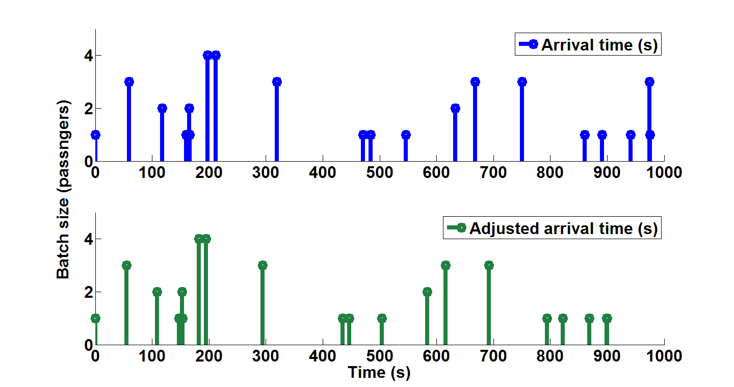
Figure 1  Initial and adjusted batch arrivals

Traffic survey data

A traffic study [5] was undertaken at a transport terminal to collect batch size data with a larger data set than in Table 1. Observers used their judgment to determine if people were travelling individually, or in groups.  1249 batches were observed, results are given in Table 2.

Table 2  Probability density function for the batch sizes

Batch size	1	2	3	4	5	6
Probability	811/1249	340/1249	71/1249	19/1249	6/1249	2/1249

The results in Table 2 yield an average batch size of 1.46.

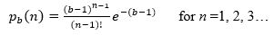
The Poisson distribution may be used to model the batch size, see Equation 1.

    (1)

Where p_b(n) is the probability of a batch size of n and b is the average batch size.  Note: it is not suggested that the underlying distribution is Poisson, but that the curve follows a similar pattern.  The classical Poisson formula is offset by 1 as there cannot be a batch size of 0.

Figure 2 shows the probability of different batch size based on measurements and as calculated using Equation 1 with an average batch size or 1.46.  The R-Squared value is 0.999 showing a good fit for the data.   At high batch sizes, Equation 1 under predicts the probability, however these instances are rare.

Figure 2 Comparison of batch size probability measured versus Equation 1

The data suggests it is reasonable for a passenger generator used by simulation software to accept input of an average batch size, then to create passenger batches assuming Equation 1.

Methodology for Generating Passengers

Introduction to the methodology

This section provides a step by step methodology for generating passengers with random inter-arrival time with an exponential probability density function. Passenger batches are selected assuming Equation 1 given an average batch size.

For example, using terminology from CIBSE Guide D Section 4 [6], consider a passenger demand represented as having an arrival rate of 24.95 person per five minutes at the entrance floor for a time period of one hour (3600 s). There are 10 upper floors with equal population resulting in a destination probability of 10% to each floor.  The average batch size, b = 1.2.

The software implementing the methodology should generate a list of passengers corresponding to the passenger demand.  All random numbers generated should be uniformly distributed.

Determining how many people to generate

With an arrival rate of 24.95 persons per five minutes, the number of passengers in this period is 12 x 24.95 persons which is 299.4 persons.

With simulation, there cannot be part passengers.  Use a random number to decide if to create 299 or 300 persons, i.e. does the person corresponding to the 0.4 turn up?

Generate a random number between 0 and 1. If the random number is ≤ 0.4, then use 300 people, otherwise use 299 people.  Assuming the random number was 0.21, the number of persons generated, Np = 300 persons.  Continue by dividing these N_p people into batches.

Generation of batches

Calculate the probability of each batch size using Equation 1. Based on an average batch size of 1.2, results are given Table 3.

Table 3  Probability density function for the batch sizes of 1.2

Batch size	1	2	3	4	5	6
Probability	0.819	0.163	0.016	0.001	0.000	0.000

Proceed as follows:

1. Generate a uniformly distributed random number between 0 and 1.
2. If the random number is ≤ 0.819, then the batch size is 1.  Otherwise, if the random number is ≤ (0.819+0.163) then the batch size is 2.  Otherwise, if the random number is ≤  (0.819+0.163+0.016) then the batch size is 3.  And so on.
3. For example, if the random number is 0.82 this will yield a batch size of 2.  There are now 300-2 = 298 people left to assign to batches.

Repeat the procedure (i) to (iii) until all 300 passengers are part of a batch.

In the final repeat of the procedure, there may not be enough people left for the batch size selected by the random number.  For example, if the random number generated calls for a batch size of 3, but already 298 people have been put in batches, then the final batch size is taken to be 2.

Call the number of batches generated Nb.  Once the passenger batches have been generated, the arrival times of the batches can be determined.

Generation of arrival times

A procedure to generate batch arrivals and random inter-arrival time with exponential probability density function as described by Peters et al [4] is summarized in Section 2.

The average batch size is 1.2 persons, and there are 300 persons. On average, there are 300 persons/ 1.2 persons per batch = 250 batches. In this example, the software generated 252 batches.  These arrive in one hour (3600 seconds).  So, the batch arrival rate λ_b is

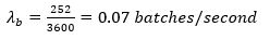 (2)

〖∆t〗_i is the inter-arrival time between batch i and batch i+1 [4]

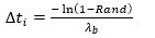(3)

for i=0 to N_b+1.  Rand is a function that generates a random number between 0 and 1.

In Section 2, Figure 1 the first passenger arriving at time = 0 s.  In the context of simulation software which may have many consecutive periods, it is preferable not to have a passenger arriving at the instant each period begins.  To address this, add half a randomly generated inter-arrival time after the period start time.  This allows multiple periods to follow each other without a person marking the start of each period, see 〖∆t〗_0 in Figure 3.

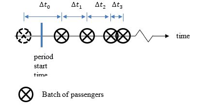
Figure 3 Placing the first batch on the time line

Continuing placing all the batches on a time line using Equation 3, see Figure 4. The period end time is only approximate as the calculation of inter-arrival times includes a random element.

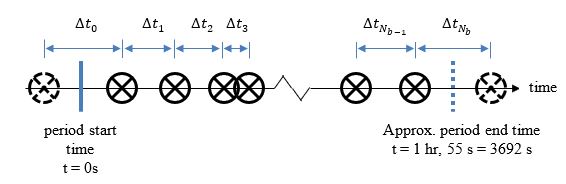
Figure 4 Passenger batches on time line

Shrink or stretch the inter-arrival times so that the batches arrive within the period.  A scaling factor, SF, can be determined by establishing the ratio between the sum of the generated inter-arrival times and equivalent time taken with passengers arriving at the batch arrival rate, λ_b, see Equation 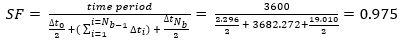4.

(4)

The adjusted inter-arrival times, ∆ts_i can then be determined, see Equation 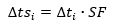5.

(5)

Apply the SF so that the batch of passengers aligns with the actual period end time, see Figure 5.

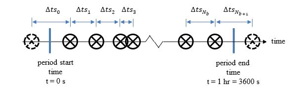
Figure 5 Passenger batches with inter-arrival time adjusted to align in actual period end time

Passenger destinations

It is assumed that each passenger batch has the same destination.  The destination probability to each floor above the entrance floor was 10% (=0.1), see Table 4.

Table 4 Batch destination probabilities

Floor	1	2	3	4	5	6	7	8	9	10	11
Destination probability	0	0.1	0.1	0.1	0.1	0.1	0.1	0.1	0.1	0.1	0.1

For each batch, generate a random number between 0 and 1.  If the random number is ≤ 0.1, the destination is floor 2.  Otherwise, if the random number is ≤ (0.1 + 0.1), the destination floor is floor 3.  Otherwise, if the random number is ≤ (0.1 + 0.1 + 0.1), then destination floor is 4.  And so on.

Example results

Passenger generation

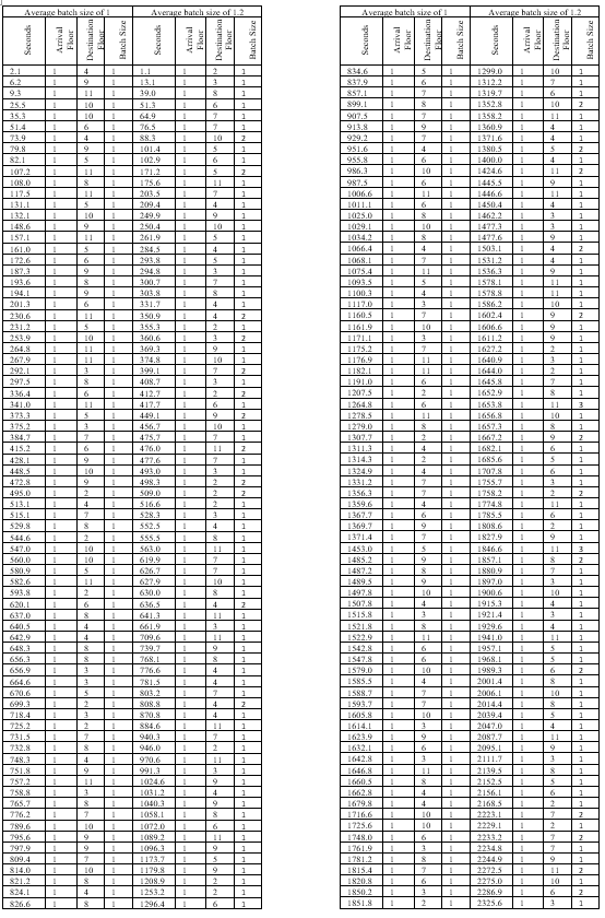
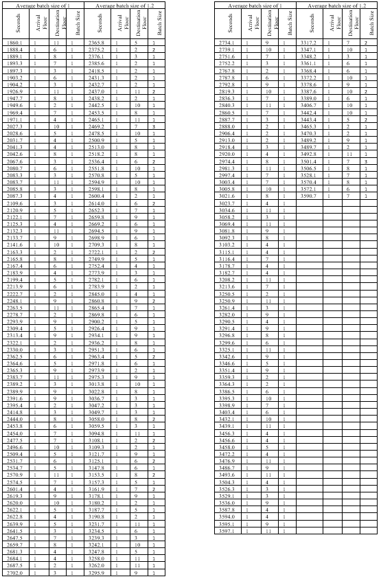
Example results for the above example with a batch size of 1.0 and 1.2 are given in Table 5.

Table 5  Example passenger generation results

  

Discussion of results

24.95 persons per five minutes yields 299.4 person in one hour.  In this example, a single run, 300 people have been generated.  With multiple runs, sometimes 299 people will be generated. As the number of runs increases, the average will tend to 299.4.

Likewise, the distribution of destinations will tend to 10% (0.1) for each floor as the number of runs increases.  Table 6 shows the distribution of destinations generated for the run with batch size 1.

Table 6 Example input and actual destination probabilities

Floor	1	2	3	4	5	6	7	8	9	10	11
Input   destination  probability	0	0.1	0.1	0.1	0.1	0.1	0.1	0.1	0.1	0.1	0.1
Generated destination probability	0	0.08	0.10	0.13	0.07	0.10	0.11	0.10	0.11	0.09	0.12

Table 7 shows the input and output probability density function of batch size for the run with average batch size 1.2.  As the individual batch size probabilities get smaller, the occurrences get rarer.  The input probability of a batch size of 4 is one in a thousand.  So, with 300 passengers generated, it is not surprising that no batches of 4 were generated.

Table 7 Example input and output probability density functions with average batch sizes 1.2

Batch size	1	2	3	4	5	6
Input probability	0.819	0.163	0.016	0.001	0.000	0.000
Output probability	0.825	0.159	0.016	0.000	0.000	0.000

Effect of batching on simulation results

In a test simulation with this sample data, the average time to destination of passengers was reduced by approximately 5 seconds with batching.  No generalizations can be made from this single run, but it does demonstrate that batching has an impact on simulation results.

In most cases batching is likely to improve waiting time in simulation, as in the real world.  This is because the stops arising from the calls are coincident; overall the number of lift stops is less.

There may be some other unexpected consequences of batching.  For example, a simulation program may, by default, assume that batched passengers insist on travelling together.  So, if the lift had space for one person and the batch was two people, they will wait for the next lift.

Conclusions and further work

Lift passengers often travel together in groups rather than alone.  For this to be reflected in lift simulation software, batches must be considered.  Batches influence simulation results as passengers travelling in groups generate less calls.

This paper provides a procedure for generating passengers including batches.  Passengers are generated assuming a random inter-arrival time with an exponential probability density function. Passenger batches are selected using Equation 1, given an average batch size.  Traffic survey data has been collected and shows a good fit to the proposed passenger generation process.  Further site data will be collected in different building types, and other batch size probability distributions may be considered.  The objective is for users to describe batching with a single number for each application.

The discussion also provides an insight into the numerous decisions a simulation software designer needs to make.  Many of these decisions are not normally considered as inputs, yet they influence simulation results.

REFERENCES

1. J. Kuusinen, J. Sorsa and M. L. Siikonen, “A study on the arrival process of lift passengers in a multi-storey office building,” BUILDING SERV ENG RES TECHNOL, vol. 33, no. 4, pp. 437-449, 2012.
2. J. Sorsa, J.-M. Kuusinen and M.-L. Siikonen, “Passenger Batch Arrivals in Elevator Lobbies,” Elevator World, January 2013.
3. N. T. J. Bailey, “On Queueing Processes with Bulk Service,” Journal of the Royal Statistical Society, Series B (Methodological), vol. 16, no. 1, pp. 80-87, 1954.
4. R. Peters, L. Al-Sharif, A. T. Hammoudeh, E. Alniemi and A. Salman, “A Systematic Methodology for the Generation of Lift Passengers under a Poisson Batch Arrival Process,” in Proceedings of the 6th Symposium on Lift & Escalator Technology, Northampton, 2015.
5. Peters Research Ltd, “Private Client Report,” 2017.
6. R. Peters, “Advanced planning techniques and computer programs,” in CIBSE Guide D, London, The Chartered Institution of Building Services Engineers, 2015, pp. 4/1-4/18.

ACKNOWLEDGEMENTS

Professor Lutfi Al-Sharif and Dr Marja-Liisa Siikonen for introducing us to some key concepts which we have applied and developed. Elizabeth Evans and Rachael Graves for managing the collection of survey data.  Tikshananshu Kumar for advice on the Poisson distribution and its suitability in the case of batching passengers.

BIOGRAPHICAL DETAILS

Richard Peters has a degree in Electrical Engineering and a Doctorate for research in Vertical Transportation. He is a director of Peters Research Ltd and a Visiting Professor at the University of Northampton. He has been awarded Fellowship of the Institution of Engineering and Technology, and of the Chartered Institution of Building Services Engineers. Dr Peters is the author of Elevate, elevator traffic analysis and simulation software.

Sam Dean is a Software Engineer with Peters Research Ltd.  He is part of the team working on enhancements to Elevate and related software projects. He is the lead developer behind the databases and servers managed by Peters Research.