
Maria Abbi, Richard Peters
Peters Research Ltd
This paper was presented at The 9th Symposium on Lift & Escalator Technology (CIBSE Lifts Group, The University of Northampton and LEIA) (2018). This web version ©Peters Research Ltd 2018.
Keywords: lift, elevator, simulation, dispatcher, Monte Carlo
Abstract. Lift simulations use a random number generator to create a list of passengers based on anticipated passenger demand. Depending on the random number seed, different lists of passengers and resulting lift journeys will occur. Each random number seed scenario yields a different simulation run with different results. An infinite number of runs would yield results including a mean average waiting time and standard deviation which would be fully representative of the data. But only a finite number of runs can be completed as there are practical limitations on time and processing resources. How many runs need to be completed until the mean average waiting time can be said to be statistically valid? Different approaches to assessing the number of runs required for statistically valid results are proposed and discussed. The preferred approach allows the user to specify the required confidence level and acceptable range. The method can be applied to both dispatcher-based and Monte Carlo simulation.
1 Introduction
1.1 Passenger generation
Simulation software creates a list of passengers based on anticipated traffic demand required by the user. Different approaches to how these passengers are generated is discussed by Peters et al [1] [2]. All approaches rely on random numbers to select passenger arrival times, origins and destinations reflecting the passenger demand.
As the use of random number generators introduces an element of chance, enough passengers need to be considered for an analysis of the average waiting time (or other quality of service parameter) to be valid. If the sample size (number of passengers) is insufficient, the results may be over optimistic or over pessimistic.
1.2 Dispatcher-based simulation
For dispatcher-based simulation, some designers propose a long simulation at constant demand to achieve sufficient sample size result. For example, the draft ISO 8100-32 suggests a simulation of at least 120 minutes, excluding the first 15 minutes and the last 5 minutes of each simulation from the results to avoid the influences of start and end effects, see Figure 1.
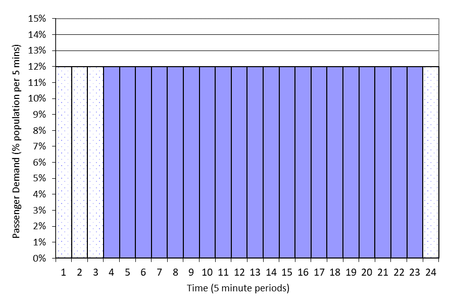
Figure 1 Passenger Demand for constant passenger demand template with first 15 minutes and final 5 minutes results disregarded
CIBSE Guide D [3] recommend designers use templates to reflect the rise and fall of passenger demand at peak times, see Figure 2, but repeat the simulation multiple times (typically 10) with different sets of passengers. Start and end effects can be disregarded as the designer reports results for just the peak 5 minutes of the profile.
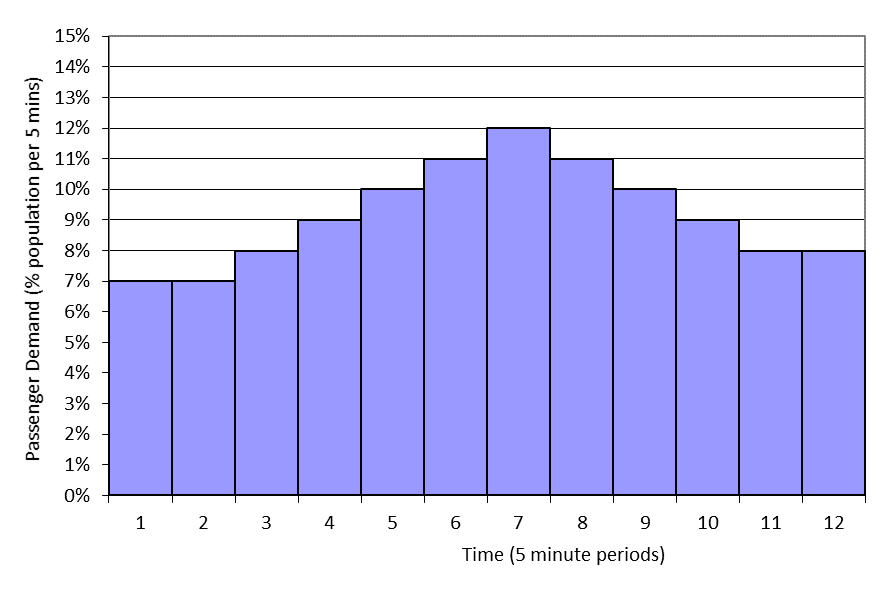
Figure 2 Passenger demand template rising and falling from peak
Both approaches work most of the time and yield relatively stable results. But sometimes 120 minutes (draft ISO 8100-32) is not long enough, or 10 simulations (CIBSE Guide D) is not enough for stability, which can be seen in counterintuitive results. For example, increasing the lift speed may increase the average waiting time. This can occur if increasing lift speed makes little difference because the travel distances are short; in which case the benefit can be so small it is lost in statistical noise.
1.3 Monte Carlo simulation
Monte Carlo simulation [4] creates a travel plan for individual round trips. Each travel plan is known as a trial. Multiple trials are completed, and an average round trip time is calculated. If enough trials are completed, the results become stable.
1.4 Objective
Running too few (or too short) simulations risks the possibility of an unrepresentative conclusion. Running too many or too short simulations is time consuming and wastes resources. This paper explores how to determine how many simulations or trials are necessary.
2 Consistent value (converging) moving average
One solution would be to take the moving average of each Average Waiting Time (AWT) result produced by each subsequent simulation. As the number of simulations, n, increases, the percentage difference between each average decreases, showing that the moving average is converging. This approach has been tested by considering 1000 simulations, 4 lifts, and up peak traffic arising from 600 people. Results are presented below.
Table 1 Moving average
| Simulation | AWT (s) | Moving average of AWT (s) | Difference |
| 1 | 6.1 | 6.1 | |
| 2 | 4.4 | 5.3 | 13.9 |
| 3 | 4.1 | 4.9 | 7.3 |
| 4 | 5.5 | 5.0 | 3.3 |
| 5 | 7.4 | 5.5 | 9.5 |
| 6 | 5.1 | 5.4 | 1.2 |
| 7 | 4.8 | 5.3 | 1.7 |
| 8 | 5.4 | 5.4 | 0.1 |
| 9 | 7.4 | 5.6 | 4.3 |
| 10 | 7.0 | 5.7 | 2.5 |
However, as seen in Table 1 and Figure 3, the moving average is subject to large variation. Because the moving average can both increase and decrease as it converges (i.e. not converging as if an asymptote), it also leaves an arbitrary decision as to how many repeated consistent values of the moving average are required before the user is confident in stating that convergence has been achieved; or, for example, what percentage difference is acceptable.
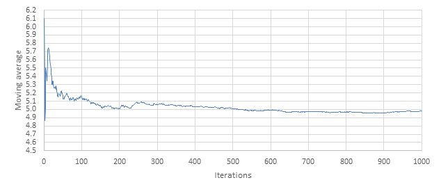
Figure 3 Moving average
The weakness of this technique is that there can be no guarantee of how representative the calculated mean is of the population. For example, consider the simulation results in Figure 3 and corresponding plot of differences in the moving average given in Figure 4: after 15 iterations the mean is 5.6 s. From 500 to 1000 simulations, the average remains around 5.0 s. However, it is quite possible that for 1000 to 2000 simulations, the mean begins to trend upwards again. Having no estimate of how likely the parameter is to be close to the population parameter is a disadvantage, because it is unknown how much confidence can be held in that result.
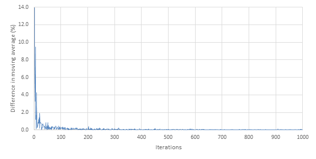
Figure 4 Difference in moving average (%)
3 Confidence intervals
3.1 About confidence intervals
In statistics, the population is the total set of observations that could be made. A sample is part of that population. In lift simulation it is not practical to consider the total set of observations. As a result, the mean cannot be determined exactly, and an estimate is needed. Confidence intervals [5] are used to determine how close the statistical estimates of the parameters of a population are to the actual population parameters and the confidence that can be held in that determination. A confidence level is the probability that the confidence interval contains the true value of the parameter.
For example, if after 10 simulations (a sample) we calculated the AWT is 5 seconds (estimate of mean), we may determine with 90% probability (confidence level) that, if we ran an infinite number of simulations (the population), the AWT would be between 3 seconds and 7 seconds (confidence interval).
There are various statistical techniques to help calculate confidence intervals and associated confidence levels.
3.2 Probability distribution
To calculation a confidence interval, probability distribution needs to be considered. A probability distribution is a “mathematical function that provides the probabilities of occurrence of different possible outcomes in an experiment” [6].
The probability distribution of AWTs determined by simulation varies for each lift configuration and set of simulation parameters (length of simulation, number of people, number of floors, number of lifts, etc.). These distributions are Lognormal (see Figure 5) rather than Normal (see Figure 6) as the AWT can never be less than or equal to 0s, whereas right tail can theoretically be infinitely long. A Lognormal distribution is “a continuous probability distribution of a random variable whose logarithm is normally distributed” [7].
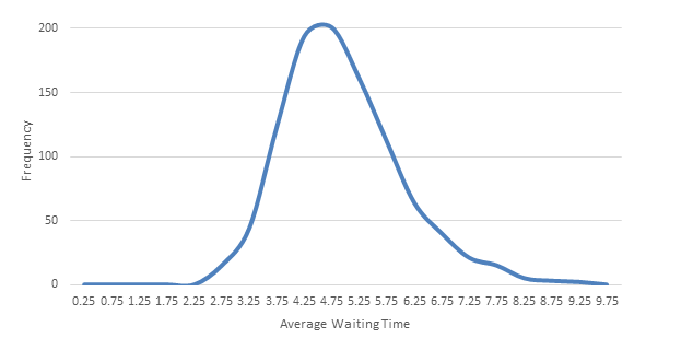
Figure 5 Distribution of AWT for simulation example
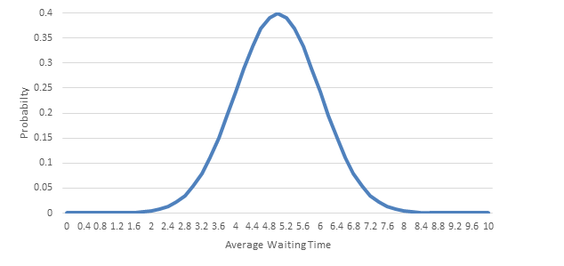
Figure 6 – Normal distribution
3.2.1 Cox method
Olsson [8] presents Cox’s method for calculating confidence intervals for data with a Lognormal distribution.
The Cox method requires that the variable x is transformed to y=ln(x), before sample parameters are calculated.
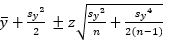 (1)
(1)
Where  is the mean of the transformed data, z is the chosen z-value (Table 2), sy is the transformed sample standard deviation and n is the number of samples.
Table 2 Confidence levels and corresponding z values
| Confidence level | ||||
| 70% | 80% | 90% | 95% | 99% |
| 1.04 | 1.28 | 1.65 | 1.96 | 2.58 |
When this is transformed back,  within an interval + or – e
  .
.
This method is only valid for large values of n and yields wide intervals. For example, with 1000 simulations and requiring at a 95% confidence interval, the results in Table 3 were obtained.
Table 3 Confidence intervals using Cox method
| Number of simulations | Mean | Upper bound | Lower bound |
| 1000 | 5 | 36.1 | 0.7 |
The Cox method was rejected as the number of simulations required to reach a satisfactory confidence interval is too high to be applied in dispatcher-based simulation.
3.3 Based on Normal distribution
If the probability distribution of AWTs can be approximated as Normal, analysis using the empirical rule [9] and confidence intervals is available.
The empirical rule requires that the mean estimation error is 0 and the distribution of errors is Normal. The D’Agostino test of Normality [10] is inconsistent in its conclusion; sometimes the example data passes the test of being Normal, sometimes it does not. For the purposes of confidence intervals, it is sufficiently close not to be rejected (Figure 5 and Figure 6) [9].
Calculation of two-sided confidence intervals is as follows:
 (2)
(2)
Where  is the mean, z is the chosen z-value, s is the sample standard deviation and n is the number of samples. Guttag states [9] that the mean, , is the population parameter within + or –
  with a certain confidence level.
As the number of samples increases, the confidence interval typically decreases. Thus the population parameters are located within a smaller margin. This can be utilised: rather than arbitrarily choosing when the results are converging on the population parameter, one decision on the width of the interval for the location of the population parameter is required. This means each simulation run can use previous simulations to calculate moving sample parameters and each subsequent confidence interval narrows down the exact position of the population parameter.
3.4 Based on t-distribution
For the first simulations, n is not sufficiently large for the Normal distribution to be used, so instead the t-distribution should be used. Sufficiently large has been determined as n > 25 [11]. Or n > 30 as shown in [12]. For the analysis t values should replace z values corresponding to certain confidence levels and degrees of freedom (v) (v=n-1) [11].
Table 4 – Confidence levels, degrees of freedom and corresponding t values
| Confidence level | |||||
| v | 70% | 80% | 90% | 95% | 99% |
| 1 | 1.96 | 3.08 | 6.31 | 12.71 | 63.66 |
| 2 | 1.39 | 1.89 | 2.92 | 4.30 | 9.93 |
| 3 | 1.25 | 1.64 | 2.35 | 3.18 | 5.84 |
| 4 | 2.13 | 1.53 | 2.13 | 2.78 | 4.60 |
| 5 | 2.01 | 1.48 | 2.01 | 2.57 | 4.03 |
Calculation of two-sided confidence intervals is as follows:
 (3)
(3)
Driels et al [11] state confidence intervals (equation 3) should be calculated with n-1 rather than n. However, this is not supported in most of the literature [12] [13] so has not been applied.
Petty [14] suggests that if the standard deviation of the population is unknown, the population standard deviation may be approximated by that of the sample and the t distribution may be used in place of normal distribution. The closeness of t values and z values in the ranges we are considering is such that the impact is too small to be worth considering for lift simulation.
3.5 Conditions for use
For analysis with confidence intervals, the statistics required that the AWT calculated in one iteration is independent of every other iteration. Waiting Times within single simulation are not independent, so this approach using confidence intervals could not be used with a long simulation at constant demand unless there were multiple long simulations.
If the lift simulation is saturated (demand exceeds handling capacity), the distribution of average waiting times will not be Normal or approximately Normal. In this case, the AWT does not need to be determined as the lift configuration should, in any case, be rejected.
4 Implementation
Inputs to dispatcher-based simulation software become:
- Acceptable range, e.g. ± 2 seconds
- Confidence level, e.g. 90%
In this case, if the calculated AWT was 5 seconds, multiple simulation would be run until the software can confirm with at least 90% confidence that the AWT is between 3 and 7 seconds. Note: the values given are only for example. The authors anticipate recommended values will be published in future design documents after discussion and review.
This is achieved as follows:
As each successive iteration takes place, the sample of AWTs increases by one. Each time the sample accumulates another AWT the confidence intervals is calculated for the chosen confidence level using the t-distribution method (up to 25 iterations) or Normal distribution method (> 25 iterations). If the confidence interval is less than the acceptable range specified by the user, the analysis is complete and the mean AWT is reported.
A similar approach can be implemented in Monte Carlo simulations using Round Trip Time (RTT) in place of AWT. RTT is assumed to meet the same criteria of Normality; there will be differing reasons for the sample not being exactly Normal, but the approximation is reasonable.
5 Conclusions
This paper reviews possible ways of choosing how many simulation iterations are necessary to provide a result within an acceptable range with a required confidence. A range of statistical techniques are presented and discussed. The chosen method approximates the population distribution of simulation results to Normal, which the authors consider reasonable and practical.
The technique proposed can be applied to both dispatcher-based and Monte Carlo simulation.
The benefit for users of simulation software is that they will no longer need to choose an arbitrary number of simulations; instead they may specify an acceptable range and confidence level that results are required to satisfy.
REFERENCES
- R. D. Peters, A.-S. L., H. A. T., A. E. and S. A., “A Systematic Methodology for the Generation of Lift Passengers under a Poisson Batch Arrival Process,” Proceedings of the 5th Symposium on Lift & Escalator Technology, 2015.
- R. D. Peters and S. Dean, “Creating Passengers in Batches for Simulation,” Proceedings of the 7th Symposium on Lift & Escalator Technology, 2017.
- R. D. Peters, “Advanced planning techniques and computer programmes,” in CIBSE Guide D: 2015 Transportation Systems in Buildings.
- A.-S. L, A. H. M and A. L. M, “The use of Monte Carlo simulation in evaluating the elevator round trip time under up-peak traffic conditions and conventional group control,” Building Services Engineering Research and Technology, vol. 33(3), no. doi:10.1177/0143624411414837, p. 319–338, 2012.
- Wikipedia, “Confidence interval – Wikipedia,” [Online]. Available: https://en.wikipedia.org/wiki/Confidence_interval. [Accessed 24 August 2018].
- Wikipedia, “Probability distribution – Wikipedia,” [Online]. Available: https://en.wikipedia.org/wiki/Probability_distribution. [Accessed 24 August 2018].
- Wikipedia, “Log-normal distribution – Wikipedia,” [Online]. Available: https://en.wikipedia.org/wiki/Log-normal_distribution. [Accessed 24 August 2018].
- U. Olsson, “Confidence Intervals for the Mean of a Log-Normal Distribution,” Journal of Statistics Education, vol. 13, no. 1, 2005.
- J. Guttag, “7. Confidence Intervals,” 2018.
- P. Marr, “Testing for Normality,” Shippensburg University, [Online]. Available: http://webspace.ship.edu/pgmarr/Geo441/Lectures/Lec%205%20-%20Normality%20Testing.pdf. [Accessed 3 April 2018].
- M. R. Driels and Y. S. Shin, “Determining the number of iterations for Monte Carlo simulations of weapon effectiveness,” Monterey, 2004.
- “Confidence Intervals for the Mean,” [Online]. Available: highered.mheducation.com/sites/dl/free/0072549076/79745/ch07.pdf . [Accessed 3 August 2018].
- W. Navidi, Statistics for Engineers and Scientists, McGraw-Hill, 2006.
- M. D. Petty, “Calculating and Using Confidence Intervals for Model Validation“.
BIOGRAPHICAL DETAILS
Maria Abbi is a Research Assistant at Peters Research Ltd on a gap year placement having studied Maths, Further Maths, Physics and Chemistry at Wycombe High School. She is commencing a course to study Aeronautical Engineering at Imperial College London in September 2018.
Richard Peters has a degree in Electrical Engineering and a Doctorate for research in Vertical Transportation. He is a director of Peters Research Ltd and a Visiting Professor at the University of Northampton. He has been awarded Fellowship of the Institution of Engineering and Technology, and of the Chartered Institution of Building Services Engineers. Dr Peters is the author of Elevate, elevator traffic analysis and simulation software.