Richard D Peters
Brunel University
Arup Research & Development
This paper was presented at ELEVCON HONG KONG 1995, The International Congress on Vertical Transportation Technologies and first published in the IAEE book “Elevator Technology 6”, edited by G. C. Barney. It is reproduced with permission from The International Association of Elevator Engineers. The paper was republished by Elevator World (April 1996) and Elevatori (May/June 1996). At the time of writing Richard Peters was working for Ove Arup & Partners, and enrolled on the Engineering Doctorate program at Brunel University. This web version © Peters Research Ltd 2009.
Abstract
In this paper the author considers lift kinematics, the study of the motion of a lift car. Ideal lift kinematics are constrained by human comfort criteria which limit the maximum acceleration and jerk (rate of change of acceleration) that are acceptable. Equations are presented which allow ideal lift kinematics to be plotted as continuous functions for any value of journey distance, speed, acceleration and jerk. Applications include generation of motor speed reference control curves. Supplementary results include journey time and formulae for use in lift traffic analysis.
LIST OF SYMBOLS
| d | Lift journey distance (m) |
| a | Maximum acceleration/deceleration (m/s2) |
| v | Maximum velocity (m/s) |
| j | Maximum jerk (rate of change of acceleration/deceleration) (m/s3) |
| D(t) | Distance travelled at time t (m) |
| A(t) | Acceleration at time t (m/s2) |
| V(t) | Velocity at time t (m/s) |
| J(t) | Velocity at time t (m/s3) |
| dmin | Minimum journey distance if lift commanded to stop immediately |
1. Introduction
Lift kinematics is the study of the motion of a lift car in a shaft without reference to mass or force. The maximum acceleration and jerk (rate of change of acceleration) which can be withstood by human beings without discomfort limits this motion. Ideal lift kinematics are the optimum velocity, acceleration and jerk profiles that can be obtained given human constraints.
Microprocessor controlled variable speed drives can be programmed to match reference speed profiles generated through the study of lift kinematics. Examples of these speed reference curves, similar to those shown in Figure 1, are sometimes presented in lift manufactures’ sales literature as a demonstration of the fast, comfortable and efficient lift transportation available for a particular drive system.
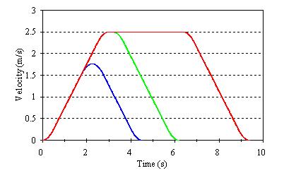
Figure 1 Example lift velocity-time profile for one, two and four floor runs
2. Overview of previous research & author’s contribution
2.1 Previous work
P D Day and G C Barney provide references of previous published work in this field in section 11.4 of CIBSE Guide D, Transportation Systems in Buildings (1). In summary:
H D Molz presented the first major work in this area in 1986. In his paper, On the ideal kinematics of lifts (2) (in German) he derives equations which enable minimum travel times to be calculated, taking to account maximum values of jerk, acceleration, and speed. If the lift trip is too short for the lift contract speed or acceleration to be obtained, the maximum speed and acceleration attained during the trip may be calculated. Some other points on the ideal kinematic curves are calculated. This paper was edited by G C Barney and re-published (3) by Elevatori in 1991 (in English and Italian).
N R Roschier and M J Kaakinen apply Molz’ formulae to provided summary tables of results for round trip time calculations (4).
In Elevator Trip Profiles (5), J Schroeder presented a computer program that calculates the maximum speed, and minimum journey time that a lift can achieve for given flight distances if there is no speed limit. This produces interesting observations such as it would take a total trip of about 17 floors for an 8 m/s lift to reach its full speed.
In Elevator Electric Drives (6) G C Barney and A G Loher suggest a computer program based on H D Molz’ equations. This is reproduced in CIBSE Guide D, Transportation Systems in Buildings (1).
2.2 Author’s contribution
The author has derived equations which allow ideal lift kinematics to be plotted as continuous functions for any value of journey distance, speed, acceleration and jerk. Supplementary results include journey time formulae for use in lift traffic analysis. The remainder of this paper is a discussion for the author’s research.
3. Derivation of ideal kinematics equations
3.1 Approach to derivation
The derivation is divided into three major sections, corresponding to the journey conditions where: (A) the lift reaches full speed; (B) the lift reaches full acceleration, but not full speed; and (C) the lift does not reach full speed or acceleration. The condition where full speed is reached before full acceleration(a2>v.j) is discarded as this would be an illogical design.
Conditions A to C are represented graphically in Figure 2. Each of the three conditions is divided into time slices, beginning and ending at each change in jerk or change in sign of acceleration. Functions of jerk were written down for each time interval, then integrated to give functions of acceleration, speed and distance over time. The end conditions of each set of functions provided the start conditions for the next time slice.
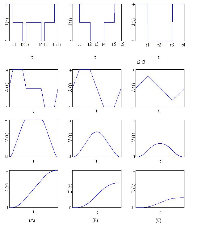
Figure 2 Ideal lift kinematics for: (A) lift reaches full speed; (B) lift reaches full acceleration, but not full speed; (C) lift does not reach full speed or acceleration
Formulae were derived to establish which of conditions (A), (B) or (C) apply given journey distance, lift speed, acceleration and jerk. The derivation is recorded in reference (7). The mathematics is relatively complex and laborious, but was aided by use of mathematical computer software (Mathcad version 4.0 from Mathsoft Inc.) which has a built in symbolic processor for equation solving.
The complete set of ideal lift kinematic equations is given in appendicies A to C. These equations may be implemented in a programming language such as Basic, Fortran, Pascal C++, etc. An example part of the derivation for condition (A) is reproduced in section 3.2.
3.2 Example section of derivation for condition (A)
Motion during time period 0 ≤ t ≤t1
For motion during time period 0 ≤ t ≤t1, referring to Figure 2(A) we can write down:
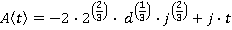
J(t) = j
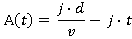
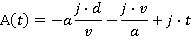
A(t) = j∙t
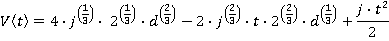
The velocity can be determined by integrating the acceleration:
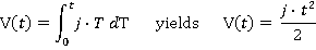
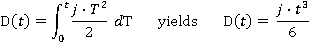
The distance travelled can be determined by integrating the velocity:
Motion during time period t1 ≤t ≤ t2, referring to figure 2(A) we can write down:
t1= a/j
J(t) = 0
A(t) = a
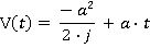
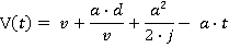
The velocity can be found by adding the velocity at the end of the previous time slice to the current acceleration, integrated:
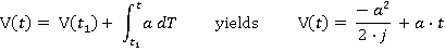
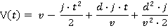
Similarly, the distance travelled can be found by adding the distance travelled at the end of the previous time slice to the current velocity, integrated:

3.3 Example results
Take journey distance, d=8 m; velocity v=2.5m/s; acceleration, a=1 m/s2, and jerk, j=2m/s2. Inputting this data into equations in appendices A to C gives us the results plotted in Figure 3. The lift reaches full speed during its journey. Calculated values of tn are: t1=0.5 s, t2=2.5 s, t3-3 s, t4=3.2 s, t5=3.7 s, t6=5.7 s, t7=6.2 s.
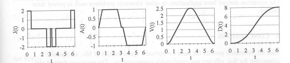
Figure 3 Example plots of jerk, acceleration, velocity and distance
4. Applications
4.1 Generation of motor speed reference curves
Motor speed reference curves are commonly held in software look up tables. It is envisaged that a software implementation of the equations presented in this paper will provide a fast, flexible and efficient way of generating optimum reference speed profiles, on line in lift system controllers.
4.2 Formulae for lift traffic analysis
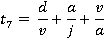
To calculate the handling capacity and performance of a lift system it is necessary to know how long it takes a lift to travel given distances. Using the appropriate formulae taken from the previous sections, the travel time of a variable speed lift (with optimum control) can be written down as follows:
If  then
then 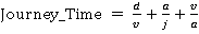 (condition A)
If 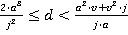 then
then 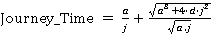 (condition B)
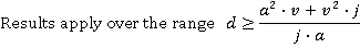
If  then
then 
 (condition C)
These equations are consistent with those presented by H D Molz[2], but are in simpler form.
It is advisable to add an additional time component to allow for motor start up time and any deviations from the optimum speed profile. Depending on drive quality, Day and Barney(1) recommend that this component should be between 0.2 and 0.5 seconds.
4.3 Other kinematic problems
The equations derived have applications to other kinematic problems such as power door control.
5. Conclusions
Ideal lift kinematics provide the basis for optimum speed control of lifts, an essential component for fast, efficient and comfortable transportation. The equations derived and presented by the author of this paper further previous research by allowing continuous , optimum functions of jerk, acceleration, speed and distance travelled profiles to be plotted against time. The results have applications in motor control and lift traffic analysis.
ACKNOWLEDGEMENTS
The author would like to thank his supervisors, lecturers and colleagues at Brunel University, Ove Arup & Partners and CIBSE Lift Group for sharing their knowledge and experience which are providing an excellent basis for research. The author acknowledges, with gratitude, financial support from the Engineering and Physical Sciences Research Council, The Ove Arup Partnership and the Chartered Institution of Building Services Engineers.
BIOGRAPHY
Richard Peters studied at Southampton University. He was sponsored by the Ove Arup Partnership and in 1987 was awarded a BSc Hons in Electrical Engineering. After graduation he joined Arup where he participated in and led the design of electrical services for a number of major, national and international construction projects. He has a special interest in Vertical Transportation and has published a number of research papers in this field. In October 1993 he joined the Environmental Technology Doctorate programme run jointly by Brunel and Surrey Universities. His project, Vertical Transportation Planning in Buildings is sponsored by Arup and CIBSE.
REFERENCES
- (Various authors) CIBSE Guide D, Transportation Systems in Buildings The Chartered Institution of Building Services Engineers (1993)
- Motz H D On the kinematics of the ideal motion of lifts Forden und haben 26 (1) (1976) (in German)
- Motz H D On the ideal kinematics of lifts Elevatori 1/91 (1991) and Elevatori 2/92 (1991) (in English and Italian) (beware typographical errors in formulae)
- Roschier N R and Kaakinen M J New formulae for elevator round trip time calculation Elevator World 28 (8) (August 1980 supplement)
- Schroeder J Elevator trip profiles Elevator World 35 (10) (November 1987)
- Barney G C and Loher A G Elevator Electric Drives Ellis Horwood, Chichester (1990)
- Peters R D Ideal Lift Kinematics: Formulae for the equations of motion of a lift (Internal Brunel University/Arup Research & Development paper)(November 1993)
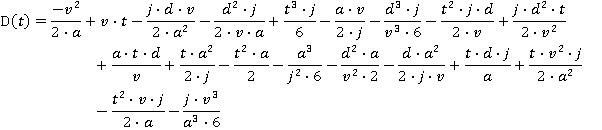
APPENDIX A Lift Reaching Full Speed During Journey


Motion during time period 0 ≤ t ≤t1
J(t) = j
A(t) = j∙t


Motion during time period t1 ≤ t ≤ t2
J(t) = 0
A(t) = a

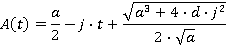
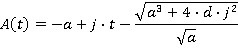
Motion during time period t2 ≤ t ≤ t3
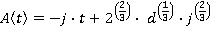
J(t) = −j
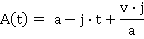

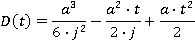
Motion during time period t3 ≤ t ≤ t4
J(t) =0
A(t) =0
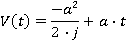
V(t) = v
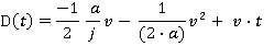
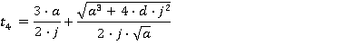
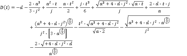
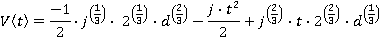
Motion during time period t4 ≤ t ≤ t5


Motion during the time period t5 ≤ t ≤ t6


Motion during the time period t6 ≤ t ≤ t7


APPENDIX B Lift Reaching Maximum Acceleration, But Not Full Speed
Results apply over the range
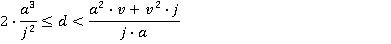


Motion during the time period 0≤ t ≤ t1


Motion during the time period t1≤ t ≤ t2


Motion during the time period t2≤ t ≤ t3


Motion during the time period t3≤ t ≤ t4

Motion during the time period t4≤ t ≤ t5

Motion during the time period t5≤ t ≤ t6

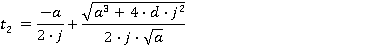
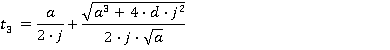
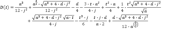
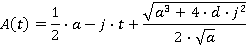
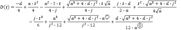
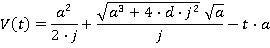
APPENDIX C Lift Not Reaching Maximum Speed or Acceleration
Results apply over the range 
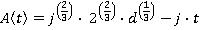
Values of tn


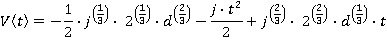
Motion during time period 0≤ t ≤ t1


Motion during time period t1≤ t ≤ t2


Motion during time period t2≤ t ≤ t3

Motion during time period t3≤ t ≤ t4