
Rosa Basagoiti, Montragon University
Maite Beamurgia, Mondragon University
Richard Peters, Peters Research Ltd
Stefan Kaczmarczyk, Northampton University
This paper was presented at Symposium of Lift and Escalator Technologies, 2012. This web version © Peters Research Ltd 2012.
Abstract
The dispatching algorithm serving in a building with more than one lift can use passenger flow detailed information based on the requests made by the passengers to go up and down in order to improve the performance of the system. The requests can be analysed in order to extract detailed information about passenger arrival and destination floors and that information used to improve lift assignments. The control strategy can be optimised to look for ways to react to changes in traffic flow. In this paper the traffic flow is described as detailed origin-destination matrixes for 5 minute time intervals. The passenger flow analysis process is divided in two steps, first passenger detailed counting and then, a forecasting process applied to the data coming from the first step. For the first step, the passenger counting process, data obtained from a typical multi-storey office building is used and the results compared with actual manual counts from the same building. After this validation process, the next step uses the data as time series where prediction methods can be applied. Prediction methods can forecast the next time interval traffic flow. Neural networks are able to approximate different time series and are used in this paper with two different data resolution entries, 5 minute interval data and 2.5 minute interval data. The results of both forecasts are compared at a resolution of 5 minutes, and the results show that a methodology of working at a higher resolution to later aggregate the result at a lower resolution can be useful in this context.Introduction
A LGCS (Lift Group Control System) serving in a building with more than one lift can use passenger flow detailed information in order to improve its performance. This information can be used to improve assignments of passenger requests to the cabs. Using detailed information about passenger arrival and destination, the optimal route selection process will be dynamically improved. With this information, the service that the system is giving to the lift passengers can be improved. It can also be helpful to understand the building needs and to improve the management of the resources it has. As an example, some lifts can be temporarily out of order or travel at different velocities according to the passenger requests and minimum service levels. It is also expected that improving the planning will move more people per time unit. This paper shows some empirical results obtained across the passenger origin destination counting process. Passengers moving through a building are manually counted and the passenger profile of the building created using ElevateTM simulation software. After this, the profile has been used to generate a log data file and this data used as an entry for an algorithm that performs the passenger counting as suggested in [1]. The validation process compares these two different passenger flows, the first coming from manual counting and the next extracted from the log data generated by ElevateTM. These two different counts are used for comparison purposes and as a validation process in order to assess the accuracy of the log based passenger counting algorithm that we have implemented. The information extracted from this first process is very detailed and can be useful for the next step, the prediction step. Although neural networks have been widely used for predicting incoming passengers and the next stopping floor, in this case, some different neural network topologies are going to be used to predict each origin and each destination of the passenger flow. We will try two different information entries to the neural network, with data at different resolutions. The output from both of the entries will be used later to validate the prediction step using data from the real count.Passenger flow and detailed counting
When the passengers travel in multi-storey building using lifts, they use the up and down call buttons of a lift system to register landing calls. These landing calls are assigned to one lift by a control unit called a lift group control system (LCGS). The information about the requests and the number of passengers boarding and alighting for each stop can be recorded and this data used to extract passenger flow patterns specific for the building. The passenger flow can be converted into origin destination matrices. These matrices show the number of passengers moving from one origin of the transportation network to a destination for a period of time. We will demonstrate an example of the information extracted for one 5 minute time interval, presented in an origin destination (OD) matrix for an 11 floor building. Each row in this matrix shows the number of passengers moving from the origin floor corresponding to the row number, to the destination floor corresponding to the column number. The matrix is first filled with 0s; the diagonal of the matrix, 0-0, 1-1, 2-2, etc. is always 0 because in a journey there is no passenger going to and from the same floor. Consider that there is a passenger on the floor 2nd who wants to travel to the 10th floor, 3 passengers travelling from floor 3rd to 9th, and 2 passengers travelling from floor 5th to 11th. If the building has 11 floors the OD matrix will be as shown in Figure 1.| 1 | 2 | 3 | 4 | 5 | 6 | 7 | 8 | 9 | 10 | 11 | |
| 1 | 0 | 0 | 0 | 0 | 0 | 0 | 0 | 0 | 0 | 0 | 0 |
| 2 | 0 | 0 | 0 | 0 | 0 | 0 | 0 | 0 | 0 | 1 | 0 |
| 3 | 0 | 0 | 0 | 0 | 0 | 0 | 0 | 0 | 3 | 0 | 0 |
| 4 | 0 | 0 | 0 | 0 | 0 | 0 | 0 | 0 | 0 | 0 | 0 |
| 5 | 0 | 0 | 0 | 0 | 0 | 0 | 0 | 0 | 0 | 0 | 2 |
| 6 | 0 | 0 | 0 | 0 | 0 | 0 | 0 | 0 | 0 | 0 | 0 |
| 7 | 0 | 0 | 0 | 0 | 0 | 0 | 0 | 0 | 0 | 0 | 0 |
| 8 | 0 | 0 | 0 | 0 | 0 | 0 | 0 | 0 | 0 | 0 | 0 |
| 9 | 0 | 0 | 0 | 0 | 0 | 0 | 0 | 0 | 0 | 0 | 0 |
| 10 | 0 | 0 | 0 | 0 | 0 | 0 | 0 | 0 | 0 | 0 | 0 |
| 11 | 0 | 0 | 0 | 0 | 0 | 0 | 0 | 0 | 0 | 0 | 0 |
- Divide the log data, for the time period needed, in our case it was 5 minutes (also 2.5 minutes for forecasting purposes).
- For a given period, separate the lift movements into journeys.
- From those journeys, the following information is collected every time the lift stops:
- Number of passengers leaving and entering the lift at each floor. To obtain this number it is necessary to have three weight measures, just before the lift arrives at the floor where it is going to stop, after the passengers leave the lift and after the lift has left the floor. The information about the number of passengers boarding and alighting can be extracted from weight sensor data or maybe the processing of camera information.
- Time stamp associated with the landing calls coming from this floor.
- Car calls that have been registered after leaving that floor.
- The principle of passenger flow conservation equation, says that the number of passengers entering and leaving a lift during a journey is equal. Using that principle, it is possible to estimate the missing information about the real passenger movements in the journey. This calculation has been done using the symbolic calculation module of MATLAB. In some cases, some rules, extra rules, are needed to be applied in order to solve the equations. These calculations are completed for all the journeys across all the lifts.
- Information about the timestamp corresponding to the first request of the journey has to be collected to later aggregate the passenger movements across all the lifts for the five minutes time intervals. The final value is obtained by aggregating from the same time interval the different journey data in one OD matrix and then, aggregating the OD matrices of the different lifts.
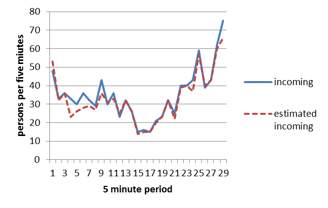 Figure 2: The number of real passengers entering the building and the estimated number of passenger incoming.
Regarding the outgoing traffic, Figure 3 shows the comparison between the real counting of the number of passengers that are leaving the building, and the estimated ones. In this case, the total number of passengers leaving the building was 1152 and we were able to detect 1087 of them, with an accuracy of 94%.
Figure 2: The number of real passengers entering the building and the estimated number of passenger incoming.
Regarding the outgoing traffic, Figure 3 shows the comparison between the real counting of the number of passengers that are leaving the building, and the estimated ones. In this case, the total number of passengers leaving the building was 1152 and we were able to detect 1087 of them, with an accuracy of 94%.
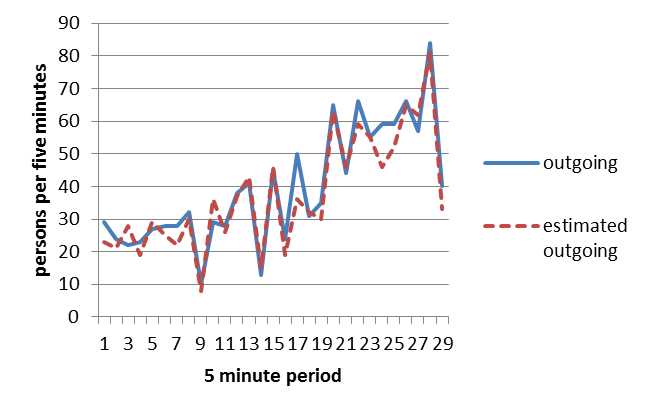 Figure 3: The number of real passenger leaving the building and the estimated number of passenger outgoing.
In order to complete the next step, the forecasting, the data has to be disposed as measures at regular intervals of time. The number of passengers moving from one floor to another (132 combination, excluding the ones that are not possible to and from the same floor), measured along the 29 intervals of 5 minutes and ordered over time are shown in Figure 4.
We have 132 different time series and 29 measures, at consecutive time intervals, for each one. The objective of this step will be to use a number h of previous time intervals for each time series to forecast the next value. As an example, one time series that represents the number of passengers moving from floor 2 to floor 6, have the next values: 6, 5, 4, 3, 0, 1. It has to be understood that 6 passengers has gone from 2nd to 6th in the first time interval, t1, 5 passengers in the next time interval, t2 and so on. Generalizing we can talk about the X time series as a sequence of values registered at regular time intervals.
X= x1,x2,x3,x4,…..,xn
Figure 3: The number of real passenger leaving the building and the estimated number of passenger outgoing.
In order to complete the next step, the forecasting, the data has to be disposed as measures at regular intervals of time. The number of passengers moving from one floor to another (132 combination, excluding the ones that are not possible to and from the same floor), measured along the 29 intervals of 5 minutes and ordered over time are shown in Figure 4.
We have 132 different time series and 29 measures, at consecutive time intervals, for each one. The objective of this step will be to use a number h of previous time intervals for each time series to forecast the next value. As an example, one time series that represents the number of passengers moving from floor 2 to floor 6, have the next values: 6, 5, 4, 3, 0, 1. It has to be understood that 6 passengers has gone from 2nd to 6th in the first time interval, t1, 5 passengers in the next time interval, t2 and so on. Generalizing we can talk about the X time series as a sequence of values registered at regular time intervals.
X= x1,x2,x3,x4,…..,xn
Forecasting
Traffic flow forecasting is the core of the transport planning and traffic control. There are a lot of forecasting methods but it is important to know the nature of the data and try to select a method that can be appropriate for the task in hand. Traffic flow data features are nonlinearity and strong interferences. The forecasting task can be tackled in different ways. Some of the methods [3] only try to train the system to identify a possible congestion with algorithmic methods. Others understand the data as a time series and use some signal processing methods [4] or box-jenkins methods [5] to do the forecasting. Support vector machines has been used also [6] for this task. A brief table, with the advantages and disadvantages of some methods can be seen in the table 1.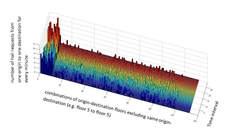 Figure 4: A bar plot of the requests for the 132 combinations (12*12 floors excluding the requests from one floor to the same) across the 29 five minute intervals.
Table 1 : Advantages and disadvantages of some forecasting methods
Figure 4: A bar plot of the requests for the 132 combinations (12*12 floors excluding the requests from one floor to the same) across the 29 five minute intervals.
Table 1 : Advantages and disadvantages of some forecasting methods
| Methods | Advantages | Disadvantages |
| Moving Average | Simple | Not Good Fit |
| Arima | Good Fit | Tedious Programming |
| Kalman Filters | Good Fit | Tedious Programming |
| Bayesian Networks | Good Fit | Tedious Programming |
| Artificial Intelligence & Neural Networks | Well Known | Fall in Local Minima |
| Support Vector Machines | Forecasting of Small Samples | Sensitive to the Selected Kernel Function |
| Wavelets & ARIMA | Wavelets have Good Decomposition Power and ARIMA Good Linear Fitting | Tedious Programming |
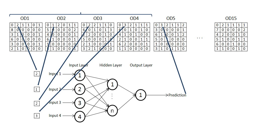 Figure 5: Structure of the Neural Network
Figure 6 shows an example of real requests coming from one origin and going to one destination, in blue, and the predicted requests for the same origin and the same destination, in red.
The methodology used for the forecasting approach was to work at two different resolution levels and to compare both sets of results. Working with detailed passenger flow data facilitates this approach because detailed data about each journey is available. Five minute interval forecasting is understood well enough to feed the dispatching algorithm. However having detailed passenger requests data for each journey, working at a low level (2.5 minutes interval or lower) and then, processing the results to obtain the desired five minutes forecasted data can be a useful approach.
The combination of more than one method has also been applied as a powerful approach, combining the better of the two methods to improve prediction accuracy.
The forecasting process must be evaluated in order to select the appropriate method. For this task, some indicators are needed to measure the quality of the method. In time series theory, three measures of the error are commonly used; MSE (mean square error), MRE (mean relative error) and MAE (mean absolute error). All of them calculate a discrepancy between the real data and the forecasted data. The equations 1, 2 and 3 show how these discrepancies are calculated. In all the equations, predictions are converted to OD matrixes, where ODij, represents the real OD matrix data for the origin-destination pairs, represented by (i,j). In the same way, ODeij is the estimated data matrix and f represents the number of floors.
Figure 5: Structure of the Neural Network
Figure 6 shows an example of real requests coming from one origin and going to one destination, in blue, and the predicted requests for the same origin and the same destination, in red.
The methodology used for the forecasting approach was to work at two different resolution levels and to compare both sets of results. Working with detailed passenger flow data facilitates this approach because detailed data about each journey is available. Five minute interval forecasting is understood well enough to feed the dispatching algorithm. However having detailed passenger requests data for each journey, working at a low level (2.5 minutes interval or lower) and then, processing the results to obtain the desired five minutes forecasted data can be a useful approach.
The combination of more than one method has also been applied as a powerful approach, combining the better of the two methods to improve prediction accuracy.
The forecasting process must be evaluated in order to select the appropriate method. For this task, some indicators are needed to measure the quality of the method. In time series theory, three measures of the error are commonly used; MSE (mean square error), MRE (mean relative error) and MAE (mean absolute error). All of them calculate a discrepancy between the real data and the forecasted data. The equations 1, 2 and 3 show how these discrepancies are calculated. In all the equations, predictions are converted to OD matrixes, where ODij, represents the real OD matrix data for the origin-destination pairs, represented by (i,j). In the same way, ODeij is the estimated data matrix and f represents the number of floors.
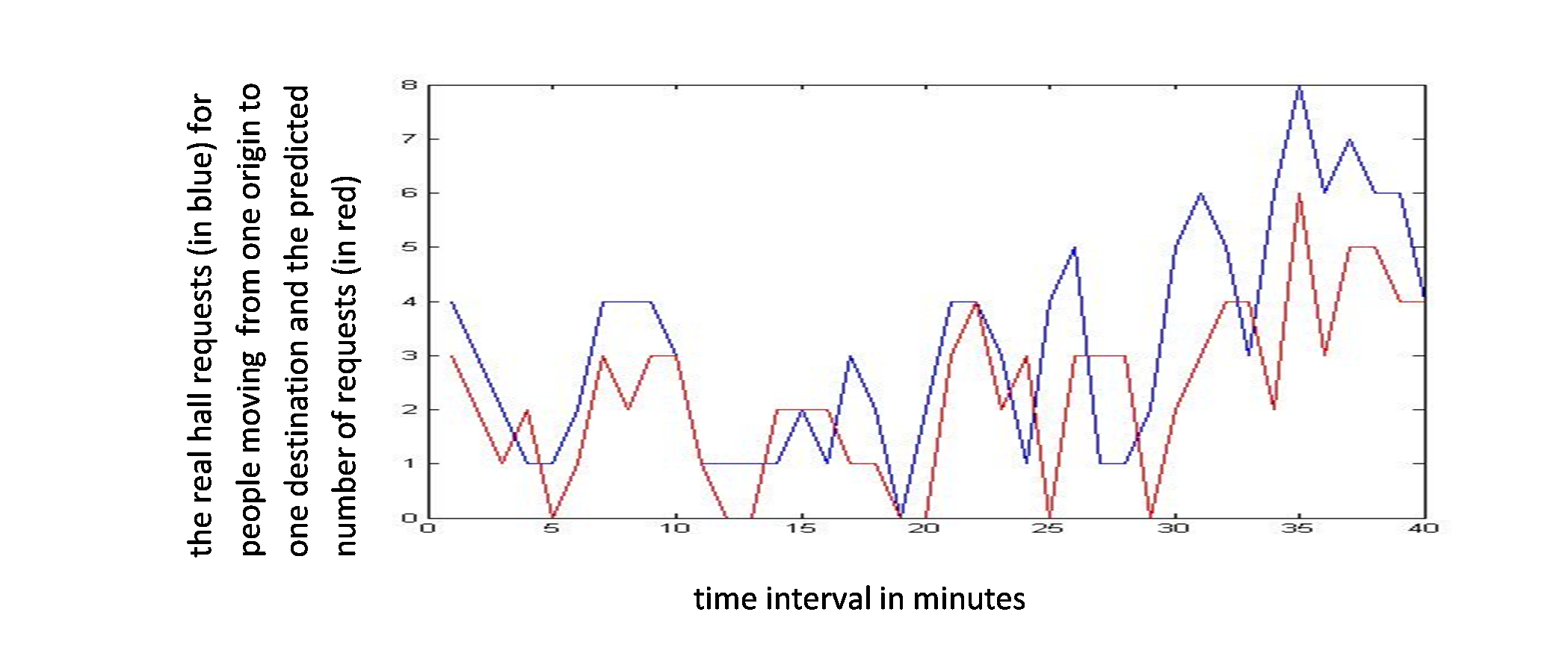 Figure 6: Passenger requests from one origin to one destination floor and the predicted requests
The first measurement is the mean square error (MSE) that describes the concentration and degree of dispersion about the error dispersion:
Figure 6: Passenger requests from one origin to one destination floor and the predicted requests
The first measurement is the mean square error (MSE) that describes the concentration and degree of dispersion about the error dispersion:
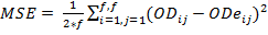 (1)
The second measurement is the mean relative error (MRE), an indicator to evaluate the whole forecasting process:
(1)
The second measurement is the mean relative error (MRE), an indicator to evaluate the whole forecasting process:
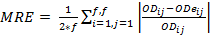 (2)
And the third measurement is the mean absolute error (MAE), the absolute average error between the predicted and actual values:
(2)
And the third measurement is the mean absolute error (MAE), the absolute average error between the predicted and actual values:
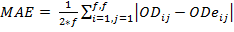 (3)
Table 2 shows the results of the three error measurements for 14 intervals. They correspond to the time period between 11:40 and 12:45. The table shows the time period, the total number of real calls for this period and the total number of predicted calls. It shows also MSE, MRE and MAE. The table also contains prediction measurements, when data about the journey for each 2.5 minutes is used to feed the neural network. The results obtained are later used to calculate the mean for the number of requests coming for each origin destination. The results are really good with this second approach. We understand that the mean calculation process can reduce the impact coming from the great variability of this data.
Table 2 : Results for the prediction step for 5 minutes interval data. 5 minutes time interval OD matrix based prediction 2.5 minutes time interval Od matrix based prediction Periods Real calls Estimated calls MSE MRE MAE Estimated calls MSE MRE MAE
(3)
Table 2 shows the results of the three error measurements for 14 intervals. They correspond to the time period between 11:40 and 12:45. The table shows the time period, the total number of real calls for this period and the total number of predicted calls. It shows also MSE, MRE and MAE. The table also contains prediction measurements, when data about the journey for each 2.5 minutes is used to feed the neural network. The results obtained are later used to calculate the mean for the number of requests coming for each origin destination. The results are really good with this second approach. We understand that the mean calculation process can reduce the impact coming from the great variability of this data.
Table 2 : Results for the prediction step for 5 minutes interval data. 5 minutes time interval OD matrix based prediction 2.5 minutes time interval Od matrix based prediction Periods Real calls Estimated calls MSE MRE MAE Estimated calls MSE MRE MAE
| 5 minutes time interval OD matrix based prediction | 2.5 minutes time interval OD matrix based prediction | ||||||||
| Periods | Real Calls | Estimated Calls | MSE | MRE | MAE | Estimated Calls | MSE | MRE | MAE |
| 11:40- 11:45 | 35 | 58 | 3,0682 | 67,42% | 0,0523 | 34 | 0,5019 | 34,47% | 0,0374 |
| 11:45- 11:50 | 31 | 49 | 1,6970 | 54,55% | 0,0302 | 32 | 0,3655 | 28,41% | 0,0163 |
| 11:50- 11:55 | 32 | 71 | 2,5076 | 73,48% | 0,0500 | 43 | 0,4754 | 30,68% | 0,0208 |
| 11:55- 12:00 | 33 | 59 | 2,2424 | 65,15% | 0,0560 | 44 | 0,4318 | 28,79% | 0,0278 |
| 12:00- 12:05 | 28 | 52 | 2,2727 | 62,12% | 0,0501 | 50 | 0,6155 | 26,14% | 0,0316 |
| 12:05- 12:10 | 47 | 55 | 3,0606 | 68,18% | 0,0710 | 47 | 0,6023 | 35,61% | 0,0420 |
| 12:10- 12:15 | 32 | 38 | 0,9242 | 34,85% | 0,0217 | 40 | 0,3902 | 23,48% | 0,0222 |
| 12:15- 12:20 | 52 | 79 | 1,9167 | 53,79% | 0,0490 | 52 | 0,5095 | 26,14% | 0,0272 |
| 12:20- 12:25 | 48 | 62 | 1,4848 | 53,03% | 0,0469 | 40 | 0,9811 | 31,82% | 0,0383 |
| 12:25- 12:30 | 50 | 35 | 2,1894 | 67,42% | 0,0489 | 48 | 0,6117 | 32,2% | 0,0309 |
| 12:30- 12:35 | 72 | 84 | 2,7576 | 72,73% | 0,0510 | 64 | 1,1420 | 39,02% | 0,0252 |
| 12:35- 12:40 | 50 | 48 | 1,5303 | 57,58% | 0,0624 | 54 | 0,4242 | 28,03% | 0,0300 |
| 12:40- 12:45 | 58 | 50 | 2,8485 | 69,7% | 0,0883 | 49 | 0,4337 | 26,89% | 0,0335 |
| 12:45- 12:50 | 79 | 42 | 3,1288 | 79,55% | 0,0586 | 57 | 0,9905 | 40,53% | 0,0243 |
| Total | 647 | 782 | 31,6288 | 8,7955 | 0,7364 | 654 | 8,4753 | 4,3221 | 0,4075 |
Conclusion
In the vertical transportation the information provided by the log of the requests and trips of the cabs, provides the possibility to perform a comprehensive movement counting between floors. This valuable information can also be used to forecast demand in the minutes after. This will allow for better planning in dispatching and also support building applications that can take advantage of it. As for the prediction, neural networks offer good fitting to variable data. The methodology for analysis at high resolution and subsequent average at lower resolution has proven effective for this type of data but subsequent tests need to confirm it. Further development will consider origin-destination matrices estimation [2] and hybrid methods [7]. REFERENCES- Juha-Matti Kuusinen, Janne Sorsa, Tuomas Susi, Marja-Liisa Siikonen, Harri Ehtamo A new model for vertical building traffic. Transportation Research. 2010.
- Li, B Markov models for bayesian analysis about transit route origin-destination matrices, 2009. Transportation Reasearch Part B 43 (3), 301-310.
- Hiri-O-Tappa, Kittipong; Pan-Ngum, Setha; Pattara-Atikom, Wasan; Narupiti, Sorawit A Novel Approach of Dynamic Time Warping for Traffic Congestion Detection and Short-Term Prediction. 17th ITS World congress, 13p. 2010.
- Hongbo Li, Yong Peng Traffic Flow Prediction Based on Wavelet Analysis and Artificial Neural Network. ICLEM: Logistic for Sustained Economic Development: Infrastructure, Information, Integration. Section: Volume IV – System Optimization and Simulation Models, pp. 3528-3534. 2010.
- Ni Lihua, Chen Xiaorong, Huang Qian ARIMA model for traffic flow prediction based on wavelet analysis. 2nd International Conference on Information Science and Engineering (ICISE), pp. 1028 – 1031.2010.
- Xiaoke Yan, Yu Liu, Zongyuan Mao, Zhong-Hua Li, Hong-Zhou Tan.SVM-based Elevator Traffic Flow Prediction . Intelligent Control and Automation, 2006. WCICA 2006.
- Mehdi Khashei , Mehdi Bijari. An artificial neural network (p, d,q) model for timeseries forecasting. Expert systems with applications. 37 (2010) 479–489.