
Rosa Basagoiti1, Maite Beamurgia1, Richard Peters2, Stefan Kaczmarczyk3
1Mondragon University
2Peters Research Ltd.
3University of Northampton School of Science and Technology
This paper was presented at The 3rd Lift Symposium on Lift and Escalator Technologies 2013 in Northampton. This web version © Peters Research Ltd 2013
Abstract
Conventional Control in vertical transportation systems may use information about passenger flows in order to estimate the number of passengers behind each landing call and to assess the destination of these possible passengers. This information supports the lift dispatching algorithm by giving it the opportunity to implement specific strategies for different circumstances. This paper proposes a new method to identify passenger flows in advance, using historical trip counting information summarized into origin destination matrices for short periods of time. Using these matrices, a clustering procedure can identify periods of homogeneous flow present in the data, learning the main traffic flow and providing a long-term view about the traffic profile in which the system is working. Real-time information about the traffic measurements extracted from the information transmitted to the dispatching algorithm can provide the short-term view. By mixing long-term and short-term information it is possible to estimate the expected values of the unknown quantities. The benefits of this process are tested against the Multiple Travelling Salesman Problem (MTSP) where the salesman corresponds to cars and the cities correspond to landing and car calls. The MTSP is the core of a stochastic bi-level optimization problem when the genetic algorithms are applied to the lift dispatching problem.
Introduction
The lift dispatching problem is a real-time optimization problem similar to high-rack warehouses and dispatching service vehicles where the assignment can change and the decision must be taken before all the information is known [1]. The decision taken by this type of system can be considered partially revocable in that assignments can be changed up to the point at which a lift starts to decelerate to serve a call. As a new request arrives, the system can compute a new schedule for the current set of requests, replace the old schedule by the new one and follow this schedule until it is finished or replaced.
With conventional control, the lift dispatching problem suffers from a lack of information. From outside the car, the landing call provides the start floor of the trip, travel direction, and landing call time, but the number of passengers, their arrival times and the destination floors are unknown. From inside the car, the destination floor is known, but the number of passengers alighting at each floor is unknown.
A common assumption can be that nothing is known about the future. Applying this assumption, one request corresponds to only one passenger and the destination of this passenger can be any floor. When a car arrives to answer a call, it may not have enough capacity to transport all the passengers, in which case the remaining passengers will re-register their call.
To avoid this, missing information can be added using the assumption that continuously operating systems should exhibit some level of repeatability. In this case, the passenger flow pattern can record this information. It is commonly accepted that a Poisson process can be used to model the arrival of passengers [2, 3]. Later research suggests that people move around and use lifts in batches. On the other hand, if we assume that passengers travelling through specific buildings follow approximately the same pattern day after day, we can take advantage of this stability. The system can analyse information about trips previously completed, looking for a passenger flow pattern [4, 5, 6, 7].
Due to the fact that fast response times are required of a dispatching algorithm, the system analysing the flow pattern can be designed as an off-line algorithm. It can perform a data extraction process and summarise passengers’ information for different trips in the same time interval giving improved estimates for the MTSP [8].
The information required is the number of passengers behind every landing call as well as their destinations. Previous work used detailed log data to extract information about the origin and destination of the passenger trips, working towards a complete information system [9].
We will introduce details of the passenger trip data counting process, the indicator and the passenger profile used to test it. Then we will show how this information can be amended in real time, assuming we have the information necessary to synchronize off-line information about the passenger flow pattern and real-time information about the people entering the system.
Passenger flow data pattern learning
Counting passenger trip data is the first step to learning the passenger pattern flow. The flow pattern will record the number of passengers moving from an origin floor to a destination floor in a given time interval. To implement this first step, a simulation tool has been applied. Simulation represents an ideal situation, not a real one, and we understand that results need to be verified in a real situation.
The methodology used to learn the passenger flow pattern is as follows:
- Select a passenger profile that includes different traffic patterns: incoming, outgoing, interfloor. Table 1 shows the profile that has been used for the simulations completed for this paper. The profile has been designed to include a range of traffic patterns. The first 4 periods represent an up-peak (majority incoming traffic). Interfloor traffic is represented in periods 5, 6, 10, 11 and a lunch peak in periods 7, 8, 9. Finally down peak (majority of outgoing) is represented by the last 4 periods.
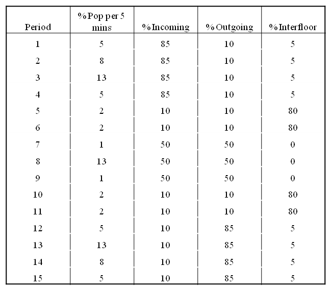
Table 1 Mixed passenger flow profile
- Execute any algorithm available in the platform 10 times with the same passenger traffic profile but different random number seeds (1 to 10), then extract a log file for the passenger trip counting process. This log is the basis of the counting. It has all the information that the passenger introduces to the system and also all the movements and data of the lifts [10].
- Extract the origin destination matrices for each log file; they will record the movements from origin to destination for every day aggregated for the considered time interval. The time interval used will be 2.5 minutes. The data obtained counting passenger trips from log data is very close to the real data and we can say that in an ideal situation, the error in the counting process is less than ± 10%. In the Eq. 1, it can be seen how to obtain the Origin Destination (OD) matrix in order to obtain the value of each floor.


Fig. 1 Comparison of the entrance data for the real and counted across OD data
- Learn a passenger flow pattern using this 10 days of information, analyse the homogeneous periods of traffic over origin destination matrices [11] and learn the traffic flow pattern [12,13]. This step has been simplified, selecting as a pattern one random day OD matrix.
- The learned pattern can be used in very different ways to feed a dispatching algorithm, one of the simplest ways to do it is by looking only at the number of people that have arrived at every floor for every time interval. It will be mixed with real time information as explained in the next sections.
- Analyse how to incorporate this information in the MTSP and measure the benefits.
Dynamically estimating passenger flow data using real time CAB load and learned pattern
The real time information [14] will be the estimated number of passengers entering the system at each floor that is recorded in a variable called Origin. The variable origin has a count of passengers that have been answered in the last 50 seconds, the interval time, for any lift. This data is separated according to the trip direction (up, down) Fig. 2.

Fig. 2 Origin data Structure
The lift stops are found for the interval time and at each stop the passenger transfers are counted. This count continues until the lifts start moving again, as shown in Eq. 2 and Eq. 3.
F: set of floors

Where q represents the load, which later is transferred into number of passengers. The direction of these trips is known because of the landing calls. The count is performed over every lift and then, summarized, and recalculated every interval time.
Mixing this real time information with the previously learned profile, will pull together long term (OD matrices aggregated for an interval time of 2.5 minutes) and short term information (Origin aggregated for an interval time of 50 seconds, a third of the long term information). Fig. 3 graphically represents what each one represents. The OD data is read from a file and Origin is calculated while the system is running. OD matrices summarize the trips expected to be performed within the time interval, whereas Origin calculates the weight entered in the system in the previous time interval. Ways to combine these can be found in the literature [15].
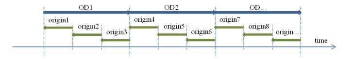
Fig. 3 Joining the OD and the Origin data
As it can be seen, the OD matrix gives future information while the origin data provides information of the recent past events. The OD data has been divided in three parts so that we can compare 3 sets of short term data with the learned profile. Before dividing the matrix, it has to be separated into up and down passenger movements as shown in Eq. 4 (up) and Eq. 5 (down). Fig. 4 represents graphically how the division of the OD is made.


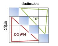
Fig. 4 OD matrix
In this way, the OD has been converted to the same style as the origin data. One side provides the number of up direction passengers and the other, the down direction passengers. This data has been converted into count the passengers moving from each floor in up or down directions. Now is possible to divide the OD in 3 parts, see Fig. 5. These 3 parts are exactly the same, because it is assumed that the passengers will arrive constantly in the 2.5 minute time interval.
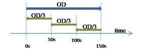
Fig. 5 Representation of the OD data in the origin format
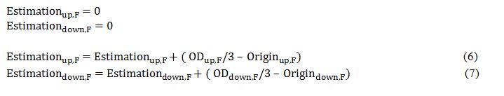
How to estimate the passengers for the next time interval
To start the estimation, the first OD is read. At this moment there is no data from the origin, so the estimation comes only from the information that can be taken from the OD. For the first interval of 50 seconds, the estimation is the value of the OD/3. After 50 seconds, an origin data set is created, so for the next estimate (from 50 seconds to 100 seconds), the origin data is taken into account. In this second estimate, we have the OD/3 value as before, but the difference between the estimation of the first interval and the actual value is added; see Eq. 6 for up direction and Eq.7 for down direction. This is used to balance the information. If most passengers from the pattern move in the first interval the second interval and maybe also the third one is consequential. The same will happen if the passengers estimated from the first interval are not as in reality.
F: set of floors
The multiple travelling salesman problem and information for the objective function
Once the passenger flow pattern has been learnt, we need to use it in real time, when the algorithm is taking the decision about which lift should serve each call. If it is assumed that nothing is known about the future, we can estimate the waiting time for the calls assigned to one lift for the MTSP as in Eq. 8, adding the different times needed for the lift to arrive and pick up a passenger waiting for it across different floors, the door close time (DCT), the runtime from the place where the lift was to the passenger’s floor, the door open time (DOT) and the transit time (DTT).
Cl: Set of landing calls

If there is some additional information about how many people can be waiting behind this landing call another term can be proposed to estimate this waiting time:

The estimation of the passengers behind a call is used directly in the MTSP. The MTSP decides the next movement of each lift, how the lifts are going to serve the landing calls. The estimation is used to give more information to the MTSP, making it easier for the MTSP to determine a better route for each lift.
But the final decision of the best route is taken with the objective function. This function can be seen in the Eq. 10.

Where EWTr is the expected waiting time of the real landing call, EWTp is the expected waiting time of the probable or the estimated landing calls, and w1, w2 are the weights of the waiting times in the objective function. w1 is for real calls and w2 for the probable or estimated calls. For all the results given in this paper the value used for w1 and w2 is equal to 0.5, giving the same weight to both function objective factors.
In the next example the improvement that can give the estimated data is explained, comparing the same situation with a MTSP with no information of the estimated passengers behind a call and a MTSP with the estimation information.
Fig. 6 shows the building that has been used for this example. The building has 21 floors and two lifts, A and B, with a maximum capacity in each of 5 passengers. There are 3 landing calls. One call on the 2nd floor that will go to the 18th floor, this call will be the 1st one. Then on the 12th floor there is another landing call, the 2nd one, and in this case it has as destination of the 20th floor. And to finish there is a 3rd landing call on the 13th floor to go to the 21st floor.
Behind the 2nd call there are 2 passengers waiting, and behind the 3rd call there are 4 passengers waiting. This data will be introduced in the MTSP with estimated passenger information.
Fig. 7 shows all the possible options the lifts have to serve the calls. For example, the 3rd possibility says that the 1st and the 3rd calls will be served by lift A and the 2nd call by lift B.
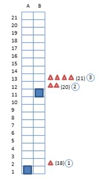

Fig. 6 The building used for the example Fig. 7 All the possible options to attend the calls
Fig. 8 and Fig. 9 show the plans for the lift in every situation, having the passengers’ data and not having it. The dark square represent the floor where the landing call has been made, and the light square the destination floor of the passengers.
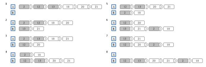
Fig. 8 All the possible plans not having passengers’ data
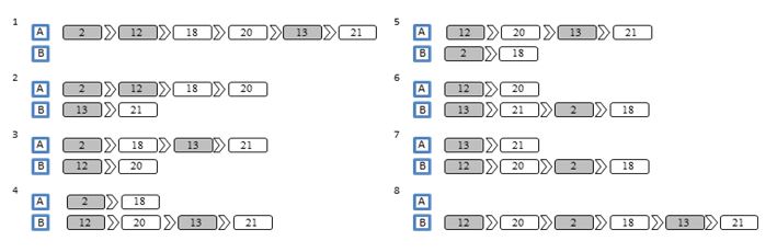
Fig. 9 All the possible plans having the passengers’ data
In Table 2, the result of the objective function is summarised, highlighting the best plan for both cases, i.e. the plan with least expected waiting time. The winner for the MTSP with no estimated passenger data is the 4th plan. The winner for the MTSP with estimate passenger data is the 2nd plan.
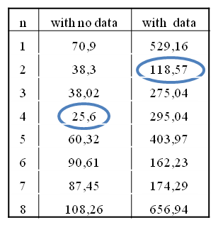
Table 2 the values of the objective function
Although the result of the MTSP, 4th plan, with no estimated passengers’ data appears to win, in reality not all the passengers will be able to enter the lift when it arrives. For example, as the lift capacity is 5 people, when the lift answers the 3rd landing call, there is not enough space for all the passengers. So the lift has to return to the 13th floor to service the passenger that could enter the first time.
In addition, the result of the MTSP with estimated passenger data penalises the plans where in the first trip the lift cannot serve all the passengers from the same call. This is one of the reasons why the expected waiting time is lower. Also, as there are some estimated passengers, the expected waiting time of those are added in the objective function, thus increasing the value. As the MTSP with the estimated passenger information better manages the capacity of the lift, the best result is different from the MTSP with no data. In this case, the winning plan is the 2nd possibility.
Conclusions
Passenger flow information can help to improve the estimation of the waiting times, thus benefiting the decisions taken in the dispatching problem. In some of our previous results, even using the simplest application of the methodology explained here, and assuming the system was filling this mixed passenger flow pattern, the benefits in the average waiting time were near 10% and the increment in the car occupancy approximately 20% for the cars at loading levels from 40% to 80%. The only measure we have noticed that has suffered from all this process is the transit time. We understand that if the lifts have to serve more people, the transit times are longer. Considering an energy aware algorithm [16], the estimation about the number of passengers waiting for the car and their destination will help in finding a better estimation of the energy consumed by each probable route.
Each step of the methodology should be reviewed with the aim of improving these initial results.
REFERENCES
[1] Benjamin Hiller, “Online Optimization: Probabilistic Analysis and Algorithm Engineering”. Operations Research Proceedings, 647-652, (2011).
[2] Richard D Peters, Pratap Mehta and John Haddon, “Lift Passenger Traffic Patterns: Applications, Current Knowledge and Measurement”. Elevcon Barcelona (1996).
[3] J.M Kuusinen, J. Sorsa, M.L. Siikonen and H. Ehtamo. “A study on the arrival process of lift passengers in a multi-storey office building”. Building services engineering research and technology, (2013).
[4] Hanif D. Sherali and Taehyung Park, “Estimation of dynamic origin-destination trip tables for a general network”. Transportation Research Part B: Methodological, Vol.35, No 3, 217-235 (2001).
[5] Sharminda Bera and K. V. Krishna Rao, “Estimation of origin-destination matrix from traffic counts: the state of the art“. European Transport, No. 49 (2011).
[6] Yuxiong Ji, Rabi G. Mishalani, Mark R. McCord, and Prem K. Goel,“Identifying Homogeneous Periods in Bus Route Origin–Destination Passenger Flow Patterns from Automatic Passenger Counter Data“. Transportation Research Board of the National Academies, Vol. 2216/2011, 42-50 (2012).
[7] Fu Guo-jiang and Pian Jin-Xiang “Study on The Lift Traffic Distribution Estimation“. Institute of Electrical and Electronics Engineers, (2012).
[8] Tapio Tyni, Jari Ylinen, “Evolutionary bi-objective optimization in the lift car routing problem”. European Journal of Operational Research, Vol. 169, Issue 3, 960-977, (2006).
[9] Zhangyong Hu, Yaowu Liu, Qiang Su and Jiazhen Huo, “A Multi-Objective Genetic Algorithm Designed for Energy Saving of the Lift System with Complete Information”. Energy Conference and Exhibition (EnergyCon), 126-130, (2010).
[10] Rosa Basagoiti, Maite Beamurgia, Richard Peters and Stefan Kaczmarczyk, “Origin Destination matrix estimation and prediction in vertical transportation”. Symposium on Lift and Escalator Technology, (2012).
[11] Yuxiong Ji, Rabi G. Mishalani, Mark R. McCord, and Prem K. Goel. “Identifying Homogeneous Periods in Bus Route Origin–Destination Passenger Flow Patterns from Automatic Passenger Counter Data”. Transportation Research Record: Journal of the Transportation Research Board, No. 2216, 42–50, (2011).
[12] Ge X and Smyth P. “Deformable markov model templates for time-series pattern matching.” Knowledge Discovery and Data Mining, 81-90, (2000).
[13] Perng C, Wang H, Zhang SR and Parker DS. “Landmarks: a new model for similarity-based pattern querying in time series databases”. 16th International Conference on Data Engineering (ICDE’2000) (2000).
[14] Pablo Cortés, Joaquín R. Fernández, José Guadix and Jesús Muñuzuri, “Fuzzy logic based controller for peak traffic detection in lift systems“. Journal of Computational and Theoretical Nanoscience, Vol. 9, No. 2, 310-318 (2012).
[15] Robert R. Andrawis, Amir F. Atiya and Hisham El-Shishiny, “Combination of long term and short term forecasts, with application to tourism demand forecasting”. International Journal of Forecasting, Vol. 27, issue 3, 870-886 (2011).
[16] Marja-Liisa Siikonen. “Effect of control systems on elevator energy consumption”. European Lift Congress, (2012).